[Edit:] fixed bottom diagram legend
Inspired by this thread, particularly by this illustration:
it occurred to me, that using a quadratic easing function you have to decide between either “smooth departure” or “smooth arrival”.
The smoothness of the movement is intuitively recognizable by the horizontal tangent at departure- or -arrival point.
What if you wanted both smooth departure and smooth arrival at both ends of a movement? You’d obviously need horizontal tangents at both ends, with a continuous (albeit not constant!) slope in between.
A Cosine function can give you just that: scaled by 0.5 in order to map the initial value range of [-1.0 … +1.0] to [-0.5 … +0.5], then vertically shifted by 0.5 gives you a value range of [0.0 … 1.0] already. Then map the input range of [-π/2 … π/2] to [0.0 … 1.0] and you’ll be set.
In case you’re wary of the performance impact of computing a trig function on every frame: a polynome of 3rd degree gives you very similar results. Someone made a quite nifty interactive cubic polynome grapher, where you can modify the A, B, C, D values of the generic cubic polynome
A * x^^3 + B * x^^2 + C * x + D = 0
via interactive sliders and immediately see the result of any change.
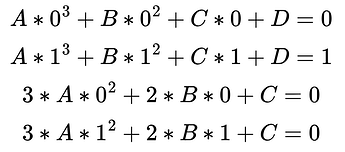
Turns out (after a little algebra), that a cubic polynome having A = -2, B = 3, C = 0, D = 0 satisfies the four boundary conditions:
- input = 0, output value = 0
- input = 1, output value = 1
- input = 0, output slope = 0
- input = 1, output slope = 0
easing.xlsx (18.4 KB)


